This and the next few blogs are about Tensorflow 2.0. I will go through a rather recent example – the cart pole game – and try to understand its advanced methods along the way.
In this blog, TensorFlow will be upgraded, some key terms will be explained and the example will be introduced.
First, the new TensorFlow version needs to be installed. With pip, this is one command prompt line:
pip install tf-nightly-2.0-preview
The usual version check shows that the upgrade worked. One of the new features of TF 2.0 is eager execution:
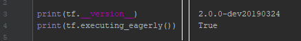
The screenshot above shows that the version has been successfully upgraded and that TensorFlow is executing eagerly. That means that computation is executed at runtime, and not in a pre-compiled graph.
Deep Reinforcement Learning
This example is about Deep Reinforcement Learning. What is that and how is it different from „normal“ Reinforcement Learning?
First, what is „normal“ Reinforcement Learning: It is an approach to solving sequential decision making problems. The AI navigates through an environment by taking actions based on observations, resulting in some form of reward. The goal is to maximize the reward by optimizing the decision making. This optimizing process is based on some algorithm, which typically takes the form of a policy the AI tries to follow. In advanced methods, the policy is a function that determines which actions should be taken in a given state. A state can be the current position of the controlled character: if the character stands before a wall (state), it should jump over it (action).
What is „deep“ Reinforcement Learning, then: An Reinforcement Learning algorithm is considered „deep“ if the policy and value functions (which are used to value an action so that the AI can get a reward) are determined by using (deep) neural networks.
Actor-Critic Methods
How does the optimization process work? There are several approaches to this; approaches that can be grouped based on their optimization methods. The so-called „Actor-Critic“ methods include:
- Value-based methods, which work by reducing error of expected state-action values.
- Policy Gradients methods, which directly optimize the policy itself by adjusting its parameters (therefore, a gradient descent algorithm is typically used). Calculating the gradients fully is often difficult – so instead they can be estimated with monte-carlo algorithms (which are a topic for the future).
- Hybrid methods, where the policy is optimized with gradients, while value based methods estimate expected values.
- Deep methods, which on top of their base functionality (may be one of the above) also use neural networks.
(Asynchronous) Advantage Actor-Critic Methods
Over many years of development, a number of improvements have been made to increase the efficiency and stability of the learning process. Some key improvements include:
- Gradients can be weighted with returns: discounted future rewards, which decrease the problem of determining the reward, and resolves theoretical issues with infinite timesteps (Q-Learning is one form of this key improvement).
- An „advantage“ function is used instead of raw rewards. „Advantage“ is the difference between a given reward and some baseline; it can be thought of as a measure of how good a given action is compared to some average action.
- An additional „entropy maximization“ term is used in the policy to ensure that the AI sufficiently explores its possibilities.
- Multiple workers can be used in parallel to speed up training by gathering and separating information about the environment.
When combining all of the improvements above with neural networks we get two of the most popular modern algorithms: (asynchronous) advantage actor critic, or A3C/A2C for short. The difference between A3C and A2C is a technical one – it is all about how the parallel workers estimate their gradients and translate them to the model.
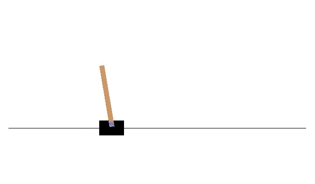
The game that follows this example is very simple – the player has to balance a pole on a cart. Implementing this example in a modern state-of-the-art way, however, requires an understanding of everything above – which is a lot of theory, with some important terms still unexplained (e.g. gradients, entropy maximzation). In the next blog, I will focus on something more practical – the implementation of the game – and (hopefully) run the first tests.
This example (the code and more information on the topic) can be found here in the source link below.
http://inoryy.com/post/tensorflow2-deep-reinforcement-learning/